How To Draw Bell Curve In Excel

A bell curve or normal distribution chart is a performance analyzer graph. Many companies use the bell nautical chart to rails the performance of their employees. Similarly, the graph can likewise be used in schools to track the performance of students. You can apply this chart to analyze the performance of a detail person in different phases or a team in a particular phase. In this article, we volition meet how to create a bell bend in Excel.

how to make bell curve in Excel

How to create a Bell Curve in Excel

To teach you the process of making a bell curve in Excel, I have taken sample data of ten students' marks in a particular subject. The marks are out of 100.

Make Bell Curve Excel Sample Data

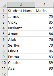
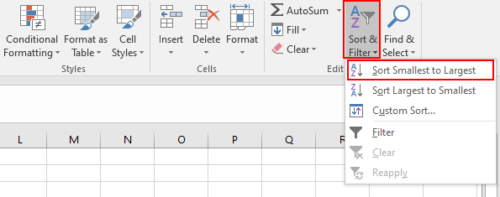
1] First, you take to arrange the entire data in ascending club. For this, select the entire cavalcade of marks, click on the "Sort Filter" button on the toolbar and select the "Sort Smallest to Largest" choice. After selecting this choice, a popup window volition appear on the screen with two options, "Expand the Selection" and "Continue with the Electric current Pick." You have to select the beginning option every bit information technology will conform the students' marks in ascending gild along with their names.

Make Bell Curve Excel Sort Data

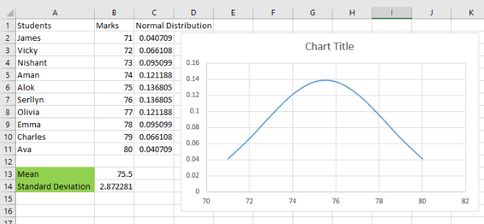
2] To create a bell curve in excel, we demand three values, average, standard deviation, and normal distribution. Let's calculate the boilerplate of the data beginning. For this, enter the following formula and press the "Enter" button:

=Boilerplate(B2:B10)

You lot tin calculate the average in any cell, I accept calculated it in B13 prison cell. Do note that yous take to enter the right cell accost in the average formula. Hither, cell B2 contains the starting time number and cell B11 contains the last number for the adding of average.

Make Bell Curve Excel Average

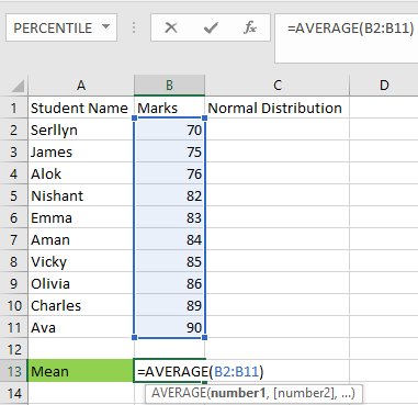
The boilerplate of our data is 82.

three] Now, allow's summate the standard deviation of the data. For this, you have to enter the following formula:

=STDEV.P(B2:B11)

Like mean, you can calculate the standard deviation in any jail cell, I accept calculated it in B14 prison cell. Again, in this formula, B2 represents the information in the B2 cell, and B11 represents the data in the B11 prison cell. Delight enter the cell address correctly.

Make Bell Curve Excel Standard Deviation

The standard deviation of our data is 6.09918. This ways that well-nigh of the students will prevarication in the range of 82 – 6.09918 or 82 + 6.09918.

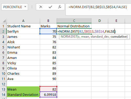
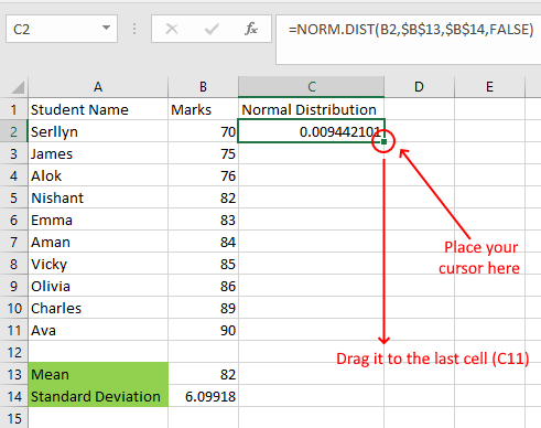
4] Now, let's calculate the normal distribution of the data. The normal distribution is to exist calculated for each student separately. Therefore, I have written it in column C. Select the cell C2 (the cell simply beneath the normal distribution cell) and enter the following formula, and press the "Enter" push:

=NORM.DIST(B2,$B$xiii,$B$fourteen,Simulated)

In the above formula, the $ sign indicates that nosotros have put the respective cell to freeze and False indicates the "Probability mass distribution." Since the bell bend is not a continuously increasing curve, we accept selected the function FALSE. The TRUE function indicates the "Cumulative distribution function" which is used to create graphs with increasing values.

Make Bell Curve Excel Normal Distribution

five] Now, place your cursor at the bottom correct corner of the selected prison cell (C2) and elevate it to the concluding cell (C11). This will copy and paste the entire formula to all the cells.

Create Bell Curve Excel Normal Distribution

6] Our data is ready. Now, we have to insert the bell bend. For this, outset, select the marks and normal distribution columns and go to "Insert > Recommended Charts."

Make Bell Curve Excel Recommended Charts

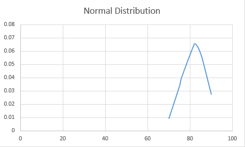
seven] At present, click on the "All Charts" tab and go to "XY Scatter > Scatter with Smooth Lines." Here, select the "Normal Distribution" chart and click the "OK" button.

Make Bell Curve Excel Insert a Chart

eight] The bell curve is ready.

Create Bell Curve Excel graph 1

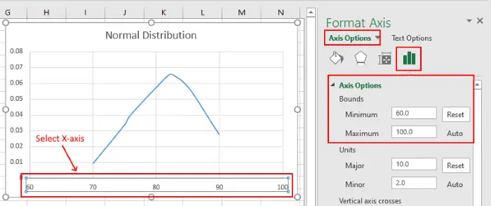
At that place are many customization options in the bell curve. You tin set the minimum and the maximum values of 10 and Y-axes past clicking on them. For your convenience, I have listed the steps to modify the values of the X-axis.

Select the 10-axis.
Select the "Axis Options" menu from the right panel and set minimum and maximum values in the "Bounds" section.

Create Bell Curve Excel graph 2

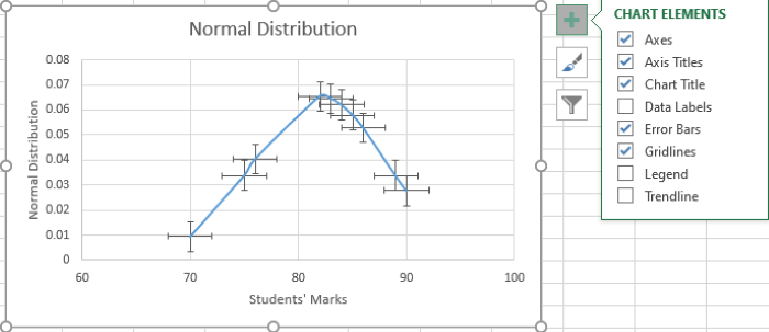
You lot can also show and hibernate different chart elements. For this, select the graph and click on the "Plus" icon. In that location, you will become a number of options. You can select and deselect any or all of them.

Create Bell Curve Excel graph Properties

Nosotros have seen in a higher place that the shape of the bell curve is non perfect. This is because the difference between the values on the X-axis (marks of the students) is not the same. At present, nosotros are creating one more than bell graph with as spaced values on the 10-axis. You take to follow the same steps mentioned higher up in the article. Meet the below screenshot.

creating bell curve in excel

This is the perfectly shaped bong curve. In this article, we accept explained the bell curve with both every bit and unequally spaced values on the Ten-centrality.

Now, you tin create a bong curve in MS excel.

You may too like: How to make a Gantt nautical chart in Excel.

how to make bell curve in Excel